flowchart LR
    S["Sales"]
    C1["Channel 1"]
    C2["Channel 2"]
    C1 & C2 --> S
    X --> C2
    C1 --> X --> S
Introduction
I came across a neat little puzzle from Quentin Gallea on LinkedIn last week (Gallea 2026). Take a marketing mix model with two channels and a third variable, X. X is a confounder for channel 2 (it drives both channel 2 and sales) and a mediator for channel 1 (channel 1 drives X, which drives sales). To identify channel 2’s effect you have to control for X. To identify channel 1’s total effect you must not, because controlling for a mediator throws away the part of the effect that flows through it. One regression can’t do both, so his conclusion is that MMMs are often too ambitious for causal estimates, and that causal inference usually goes one treatment at a time.
The diagnosis is right, and the puzzle shows up in a lot of MMM projects. A textbook case of X was given in the comments, i.e., branded search volume. Upper-funnel channels like TV make people search for your brand, so branded search volume is a mediator for TV. It also confounds anything whose budget reacts to it, and another guy pointed out in the same thread that budgets do react, because marketers scale spend up when they expect demand to be strong.
I think the conclusion is too pessimistic, though. The trouble comes from asking a single regression equation to answer two questions. Give X its own equation, give the budget rule its own equation, fit them together with sales, and then do the accounting. Both effects come back out of one model. I’ll demonstrate it with a small simulation in
Along the way the same accounting sorts out a second problem that comes with the branded search example, which is what to do with the money you spend on branded paid search. Most of it buys clicks you would have got for free, and treating it as a channel is how a lot of MMMs end up telling you branded search is your best investment.
The setup
Ok so let’s make it concrete. Channel 1 is TV. X is branded search volume. Channel 2 is paid social, and the media planner sets its budget from search trends: when branded search goes up, the social budget goes up.
A branded search lands on a results page. If you bid on your brand keyword, your ad sits at the top and your organic listing sits under it. A click on the organic link is free. A click on the ad costs you the price per click (CPC). Some searchers click a competitor’s ad instead, and those are lost. Whether you bid changes the split. With the bid on, most people click the ad. With it off, most of them click the organic link instead.
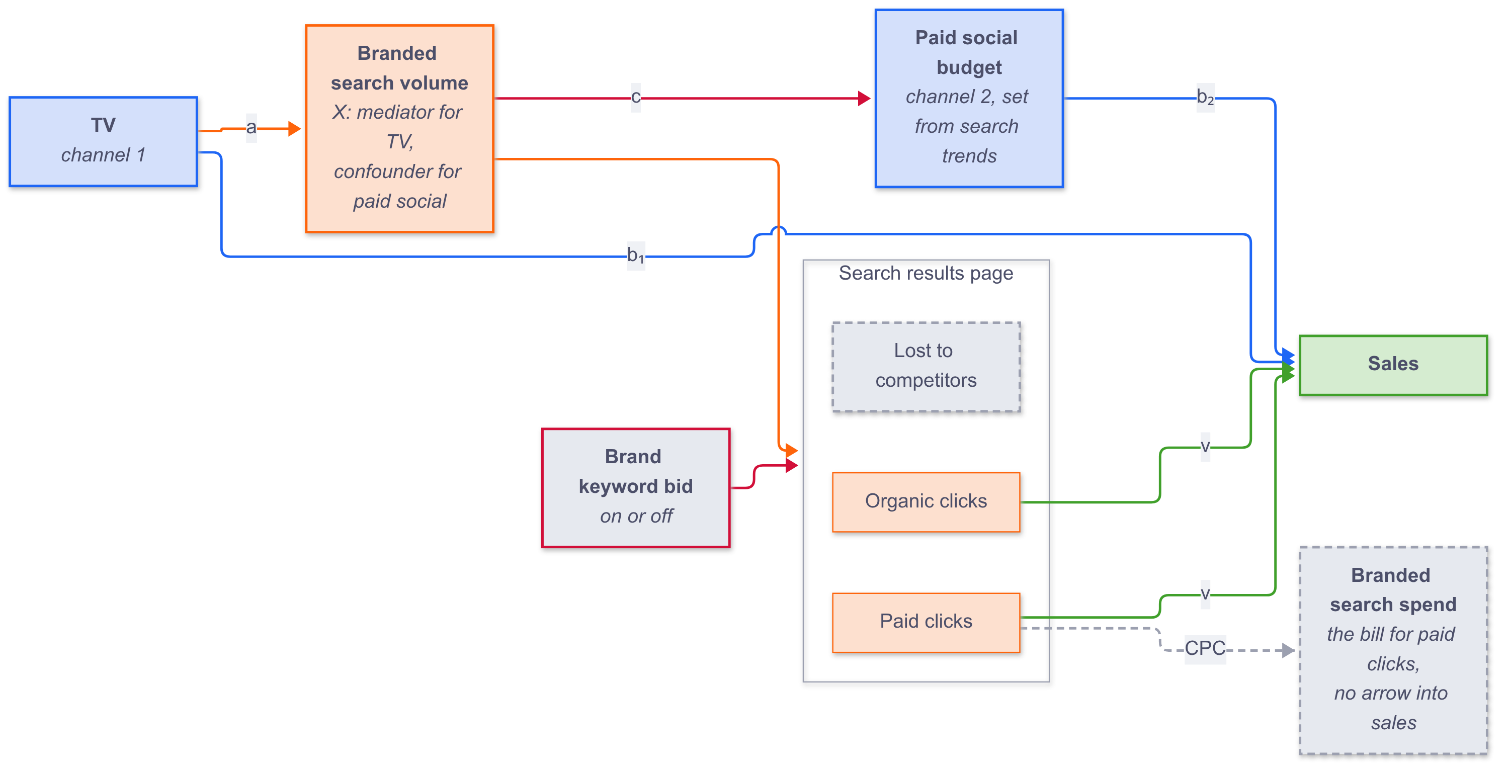
For now, assume the bid stays on, so the click split is fixed and every branded search is worth the same in sales on average. Call that \(b_x\). It’s \(v\) times the share of searches that end in a click on your result, paid or organic. Written as equations, with everything linear to keep the maths simple and boring:
\[ \begin{aligned} X &= \alpha_x + a \cdot \text{TV} + \varepsilon_x \\ \text{social} &= \alpha_2 + c \cdot X + \varepsilon_2 \\ \text{sales} &= \alpha_s + b_1 \cdot \text{TV} + b_2 \cdot \text{social} + b_x \cdot X + \varepsilon_s \end{aligned} \]
The usual MMM writes down only the last line and asks its coefficients to be the answer. Quentin’s point is that \(b_1\) is TV’s direct effect only. Everything TV does by making people search is sitting in \(b_x\) and \(b_2\), so if you report \(b_1\) as “TV’s effect” you undersell TV. Drop X from the regression to try to fix that and paid social picks up X’s effect on sales, because X moves both of them, so you oversell paid social instead.
Two questions, one equation
But why does the single equation fail? Because “what does TV do to sales?” and “what does paid social do to sales?” are questions about different interventions, and one set of regression coefficients answers one conditioning set.
For paid social, the question is: if I change the social budget and leave everything else alone, what happens to sales? Search volume doesn’t respond to the social budget in this graph, so the answer is \(b_2\), read with X in the model. Conditioning on X is exactly right here.
For TV, the question is: if I add a unit of TV, what happens to sales once you count everything downstream of TV? TV moves sales directly (\(b_1\)). It also moves search volume by \(a\), and each unit of search volume moves sales by \(b_x\). If the planner keeps following search trends, that extra search volume also moves the social budget by \(c\), which moves sales by \(b_2\). Add the paths up:
\[ \text{TV total} = b_1 + a \cdot \left(b_x + c \cdot b_2\right) \]
If you’d freeze the social budget while you add TV, the last term goes away and the total is \(b_1 + a \cdot b_x\). Those are two different questions, and the model makes you say which one you’re asking, which I count as a feature. One is about TV. The other is about TV plus the planner’s habits.
This is path tracing, and it’s old. Sewall Wright worked it out for the coat patterns of guinea pigs a hundred years ago (Wright 1920, 1921). In a linear model without interactions the total effect is the sum over directed paths of the products of the coefficients along each path, and Pearl’s do-calculus says the same thing in more general language (Pearl 2009). It’s rarely written into an MMM, though.
A simulation
Ok fine, but does it actually work? Let’s simulate three years of weekly data from the graph above, where we know the truth, and see what each approach recovers. The bid is on in every week except eight, where it’s switched off at random as a holdout test.
const a, c        = 0.8, 0.6     # TV -> branded searches, searches -> social budget
const b1, b2      = 1.0, 0.5     # direct effects on sales of TV and paid social
const v           = 1.5          # sales per click on your result, paid or organic
const cpc         = 0.5          # price of a paid click
const share_paid  = (on = 0.60, off = 0.00)   # where branded searches end up,
const share_org   = (on = 0.38, off = 0.95)   # with and without the bid

function simulate(n; sd_social = 1.0, holdout = 8)
    bid    = trues(n); bid[randperm(n)[1:holdout]] .= false   # weeks with bidding switched off
    tv     = 10 .+ 2 .* randn(n)                              # TV spend
    search = 5 .+ a .* tv .+ randn(n)                         # branded search volume
    social = 2 .+ c .* search .+ sd_social .* randn(n)        # paid social budget, set from search trends
    sp     = ifelse.(bid, share_paid.on, share_paid.off)
    so     = ifelse.(bid, share_org.on, share_org.off)
    paid   = sp .* search .+ 0.05 .* randn(n) .* bid          # paid clicks
    org    = so .* search .+ 0.05 .* randn(n)                 # organic clicks
    brand  = cpc .* (1 .+ 0.05 .* randn(n)) .* paid           # branded search spend
    sales  = 20 .+ b1 .* tv .+ b2 .* social .+ v .* (paid .+ org) .+ 2 .* randn(n)
    (; bid, tv, search, social, paid, org, brand, sales)
end
Spend and sales are in the same currency, so a coefficient on a spend variable reads as sales per euro. With the bid on, 98 percent of branded searches end in a click on your result, so \(b_x = 1.5 \times 0.98 = 1.47\), and the truth is:
- Paid social: 0.50 per euro.
- TV, direct only: 1.00.
- TV total with the social budget frozen: \(1.0 + 0.8 \times 1.47 = 2.18\).
- TV total with the social budget following search: \(1.0 + 0.8 \times (1.47 + 0.6 \times 0.5) = 2.42\).
- Branded search spend: 0.15 of sales per euro. Switching the bid off moves the paid clicks to the organic link and loses 3 percent of searches to competitors, so the ad buys 0.045 of sales per search and costs 0.30.
Now fit the usual suspects. One dataset can get lucky or unlucky, so the table averages each estimate over 2,000 simulated datasets of 156 weeks.
| Model | TV | Paid social | Branded search spend |
|---|---|---|---|
| Truth | 2.18 (social frozen) or 2.42 (social follows search) | 0.50 | 0.15 |
| sales ~ TV + social | 1.87 | 1.15 | |
| sales ~ TV + social + branded spend, bid never off | 1.31 | 0.74 | 3.11 |
| sales ~ TV + social + X | 1.00 | 0.50 | |
| sales ~ TV | 2.42 | ||
| Joint model, then the accounting | 2.18 / 2.42 | 0.50 | 0.15 |
The first row is the standard MMM that leaves search volume out. Paid social comes out at 1.15, more than double its real effect, because it’s soaking up what branded search does on its own. TV comes out at 1.87, which isn’t the right answer to either TV question.
The second row is the one I see most in the wild, and it’s the worst of the lot. Branded search spend goes in as a channel, and because it moves with search volume it soaks up a good part of what search volume does. It reports 3.11 of sales per euro, twenty times the truth, which makes it the best channel in the model by a mile. TV drops to 1.31 per euro and looks like the channel to cut. Run the same regression on data that includes the eight holdout weeks and the branded coefficient falls to 0.50, which shows how much a few weeks of switching it off are worth, but that’s still more than three times the truth.
Put search volume itself in (third row) and paid social is fixed, while TV collapses to its direct effect of 1.0, which is Quentin’s point exactly. Regress sales on TV alone and you get 2.42, the right total under the planner’s rule. That’s the one-treatment-at-a-time approach, and it works, but you need a separate model for every question you want to ask.
The joint model gets all of it from one fit. Give every node in the graph its own equation, then add up the paths:
coef(y, cols...) = hcat(ones(length(y)), cols...) \ y

â = coef(search, tv)[2]                          # TV -> search
ĉ = coef(social, search)[2]                      # search -> social budget
ŝp, ŝo = search[bid] \ paid[bid], search[bid] \ org[bid]   # click shares, bid on
_, b̂1, b̂2, v̂ = coef(sales, tv, social, paid .+ org)

b̂x         = v̂ * (ŝp + ŝo)                       # sales per branded search, bid on
tv_frozen  = b̂1 + â * b̂x
tv_follows = b̂1 + â * (b̂x + ĉ * b̂2)
social_eff = b̂2
(The real thing in the code does this inside every posterior draw, as the next section explains, and adds the bid-off share and the CPC.) Averaged over the 2,000 datasets it lands on 2.18, 2.42 and 0.50. You also get the decomposition for free. Of TV’s 2.42, 1.0 is direct, 1.18 comes through the people who search for you and click your result, and 0.24 comes through the social budget the planner adds when search goes up. That last slice belongs to TV and the planner jointly, and in the single-equation MMM paid social gets to claim it.
Where the uncertainty goes
A point estimate from a model is only half the story (yes, I know I rant about uncertainty all the time). The accounting has to carry the uncertainty through as well, because \(\hat a \cdot \hat b_x\) is a product of uncertain numbers.
The Bayesian way is to do the accounting inside every posterior draw. Take a draw of all the coefficients, compute the total effect, repeat, and you have the posterior of the total effect.
And here the linear toy gives us a nice bonus. The equations have independent noise, and if their priors are independent too, the joint posterior factorizes into one posterior per equation. So fitting regression by regression is the full joint Bayesian model, with no approximation. Put a conjugate Normal-Inverse-Gamma prior on each equation and every posterior has a closed form, so you can sample it exactly without any MCMC:
# σ² ~ InvGamma(a0, b0),  β | σ² ~ Normal(0, σ² v0 I)
function nig_posterior(y, cols...; v0 = 100.0, a0 = 1.0, b0 = 0.01, intercept = true)
    Z  = intercept ? hcat(ones(length(y)), cols...) : hcat(cols...)
    Λn = I / v0 + Z' * Z                      # posterior precision (per σ²)
    mn = Λn \ (Z' * y)
    an = a0 + length(y) / 2
    bn = b0 + (y' * y - mn' * Λn * mn) / 2
    (m = mn, L = cholesky(Symmetric(inv(Λn))).L, a = an, b = bn)
end

# Gamma(k, 1) for k a multiple of 1/2, standard library only
gamma_draw(k) = sum(randexp(floor(Int, k))) + (isinteger(k) ? 0.0 : randn()^2 / 2)

function draw(post)
    σ² = post.b / gamma_draw(post.a)
    post.m .+ sqrt(σ²) .* (post.L * randn(length(post.m)))
end
(Yes, that Gamma sampler is a sum of exponentials. With \(a_0 = 1\) every posterior shape here is a whole number or a half, so it’s exact, and it saves pulling in Distributions.jl for one line.) Then 4,000 draws go through the accounting. On a single 156-week dataset:
| Quantity | Truth | Posterior mean | 90% interval |
|---|---|---|---|
| TV total, social frozen | 2.18 | 2.05 | 1.85 to 2.26 |
| TV total, social follows search | 2.42 | 2.28 | 2.10 to 2.46 |
| Paid social | 0.50 | 0.51 | 0.22 to 0.80 |
| Branded search, sales per euro | 0.15 | 0.15 | 0.11 to 0.18 |
All four intervals contain the truth, and the TV estimates sit a little low because this dataset drew low on TV’s direct effect (0.93) and on how many searches TV creates (0.77). That’s one dataset. Over 2,000 simulated datasets the 90 percent intervals for every quantity in this post contain the truth between 88 and 91 percent of the time, which is about what a 90 percent interval should do.
The paid social interval is wide, and that’s worth a pause. The social budget follows search volume closely, so the data has little social movement that isn’t also search volume movement. In the simulation, halving the independent variation in the social budget doubles the spread of its estimate across datasets (from 0.16 to 0.32). The model is identified, but it can only be as precise as the data lets it be. If you want a tight number on paid social, this is where you run a holdout test and feed the result in as a prior, because no amount of modelling can create variation that isn’t in the data.
Branded search is mostly free clicks you pay for
Back to the results page. Why would branded paid search spend drive sales? The spend is the number of paid clicks times the CPC, and the paid clicks come from people who typed your brand name into Google, which means they were already looking for you. With the bid on, 60 percent of them click the ad and 38 percent click the organic link right under it. With the bid off, 95 percent click the organic link. So the ad mostly moves clicks from the free link to the paid one, and the only sales it adds are the 3 percent of searches it keeps away from competitors.
That’s the eBay result. eBay switched off its brand keyword ads and found that almost all of the traffic came back through organic search (Blake et al. 2015). The simulation bakes in the same story, and a regression of sales on branded spend still calls it the best channel in the model, because spend goes up exactly when demand goes up.
In the joint model the spend gets its own equation, which is the bill (CPC times paid clicks), and the bid gets to decide the click split. The data that pins down the split without the bid is the eight holdout weeks. Without them the model can tell you how clicks split with the bid on, but it can’t tell you where they’d go with it off, and you’d be back to guessing. With them, the accounting gives the value of the bid directly:
\[ \text{bid value per branded search} = v \cdot \left(s_\text{paid} + s_\text{org} - s_\text{org}^\text{off}\right) - s_\text{paid} \cdot \text{CPC} \]
Here that’s \(1.5 \times (0.60 + 0.38 - 0.95) - 0.60 \times 0.5 = -0.255\), and the joint model gets \(-0.26\) (90% interval \(-0.27\) to \(-0.25\)) on the single dataset. Every branded search with the bid on costs a quarter of a euro more than it brings in. The break-even is easy to read off: the bid pays for itself when switching it off would lose more than \(s_\text{paid} \cdot \text{CPC} / v = 0.6 \times 0.5 / 1.5 = 20\) percent of branded searches to competitors. If competitors bid hard on your name, that can happen, and the same accounting will tell you to defend it.
So the model never treats branded search as a budget line you can turn up, and that’s correct. You can’t buy more branded clicks than there are people searching for your brand. The bill rises with demand, or because you raised your bids and the CPC went with them. What the model can recommend is a bidding policy: bid where switching off would leak more than the break-even share, and don’t bid where it wouldn’t.
That changes how branded search should sit in a budget optimizer. It’s a cost that moves with demand while you bid, and that matters for every other channel. When the optimizer adds TV, TV lifts branded searches, and with the bid on you pay for the 60 percent of those searches that click the ad. The same path tracing that gives TV’s total effect on sales gives its total effect on cost:
\[ \text{TV cost per euro} = 1 + a \cdot \left(s_\text{paid} \cdot \text{CPC} + \text{follow} \cdot c\right) \]
where follow is 1 if the social budget follows search and 0 if it’s frozen. With the bid on, every euro of TV costs another 0.24 in branded clicks, and another 0.48 in paid social if the planner follows search trends. Put the sales and the costs together and the return on TV depends on both policies:
| Return per euro of TV | Social frozen | Social follows search |
|---|---|---|
| Bid on | 1.75 (joint model 1.76) | 1.40 (1.41) |
| Bid off | 2.14 (2.15) | 1.61 (1.61) |
Switching the bid off costs TV 3 percent of the searches it creates and takes away the toll it pays on 60 percent of them, so TV’s return goes up in both columns.
Compare that with the second row of Table 1. The single-equation MMM credits branded search with 3.11 per euro of sales that come from people searching for you, many of them sent by TV, and charges TV nothing for the branded clicks it causes. It undersells TV’s sales, ignores the clicks TV pays for, and points the budget at the line in the model that’s worth 0.15. Google’s own Meridian guidance models brand keyword campaigns as a channel on clicks, with a response curve and an ROI like any other channel (Google 2026). Google sells those clicks.
Disclosure: I build Alviss, a Bayesian MMM platform that competes with Meridian.
What changes in a real MMM
My toy is linear, and real MMMs aren’t. Media effects carry over (adstock) and saturate, and once you have curves the product-of-coefficients shortcut stops being exact. The principle survives, but the accounting becomes a simulation. To get TV’s total effect you take each posterior draw, bump TV spend, push the bump through the search equation, the click split, the budget rule and the sales equation, and compare predicted sales (and predicted cost) with and without the bump. That’s an intervention computed on the model. The saturation curves also break conjugacy, so the closed-form posterior goes out the window and you’re back to MCMC in a probabilistic programming language, but the accounting is still a few lines more than the linear version. It also handles timing properly: TV this week lifts search over the next few weeks, and the clicks, the bill and the planner’s response follow over the same weeks.
The data for the click split is usually available already. Paid clicks come from the ads platform, and organic clicks on your brand terms come from Search Console. What’s almost never available is the bid-off share, because almost nobody switches the bid off. A few weeks of holdout, or a geo split, is cheap and it’s the one experiment this model can’t do without.
The model also grows in a fairly natural way. With several markets or brands, each equation gets its own coefficients per market, partially pooled towards a shared mean, so a small market with noisy search data borrows strength from the larger ones. That’s the same hierarchy most Bayesian MMMs already have on the sales equation, applied to the other equations as well.
And Quentin’s worry about ten channels? It’s a fair worry. With ten channels you have more of these structures, possibly in conflicting directions. But the fix scales: each variable that something else depends on gets an equation, and the accounting is still path tracing over the graph. What doesn’t scale is writing a separate one-treatment model for every channel and hoping their answers add up to the sales you actually observed. A joint model forces them to.
The parts this doesn’t fix
This works if the graph is right, and that’s a big if. Three things will break it.
First, unobserved confounding between search volume and sales. In my simulation the extra noise in search volume affects sales only through the clicks. In real life, seasonal demand drives both branded search and sales directly (people search for your brand in December because they were going to buy in December anyway). If you don’t model that demand, \(v\) is too large and TV’s indirect effect is overstated with it. Seasonality, price, promotions and macro all need to be in the sales equation and the search equation.
Second, getting the arrows wrong. If paid social actually drives some of the branded search volume (people see the ad and then search), there’s an arrow from paid social to X, and the accounting has to include it. You need to decide the direction from what you know about the business, because the data alone usually won’t tell you.
Third, the estimand. “TV’s effect” is ambiguous until you say what happens to everything else when you change TV. Does the planner keep following search trends? Is the bid on? The model will happily give you every answer, but someone has to decide which question the business is asking. In my experience this is where most of the real arguments happen.
Conclusion
Quentin is right that a single regression can’t serve a variable that confounds one channel and mediates another. The answer is to stop asking one equation to do the work of several. Give the confounder its own equation, give the budget rule that responds to it its own equation, give the results page its own equation, fit them together, and get each causal effect by tracing paths through the fitted model. In the simulation that recovered TV’s total effect under both budget rules, paid social’s effect and the value of the brand keyword bid, from one model, with calibrated intervals. The same accounting stops branded search spend from claiming TV’s sales, and charges TV for the branded clicks it causes for as long as you keep paying for them.
It’s still only as good as the graph you draw and the variation in your data, and some numbers (paid social here, where clicks go without the bid in general) need an experiment to pin them down. But the “often not causal” part comes from how MMMs are usually specified, and the specification is yours to change. The Julia code is short, so it should be easy to wrap your head around (model, conjugate regression, accounting, one dataset, 2,000 datasets, the bid never off, coverage). Take it, break it, add the arrow from paid social back to branded search, and see what happens. And if you spot a mistake, reach out and tell me.
References
Blake, Thomas, Chris Nosko, and Steven Tadelis. 2015. “Consumer Heterogeneity and Paid Search Effectiveness: A Large-Scale Field Experiment.” Econometrica 83 (1): 155–74.
Gallea, Quentin. 2026. “Why Is Marketing Mix Modeling (MMM) so Often Not Causal?” https://www.linkedin.com/feed/update/urn:li:share:7516025366390628352/.
Google. 2026. “Meridian: Paid Search Modeling.” https://developers.google.com/meridian/docs/advanced-modeling/paid-search-modeling.
Pearl, Judea. 2009. Causality: Models, Reasoning, and Inference. 2nd ed. Cambridge University Press.
Wright, Sewall. 1920. “The Relative Importance of Heredity and Environment in Determining the Piebald Pattern of Guinea-Pigs.” Proceedings of the National Academy of Sciences 6 (6): 320–32.
Wright, Sewall. 1921. “Correlation and Causation.” Journal of Agricultural Research 20 (7): 557–85.