Introduction
I have spent an unreasonable fraction of my career being annoyed at deterministic models. They give you a number. One number. The number is wrong, almost always, and the model has no way of telling you it knows the number is wrong.
Time series is where this hurts the most. You have a stock return, a drug concentration in plasma, a sensor on a wind turbine, a river gauge, a sales effect from media. The future is always uncertain. You want a model that honors that. Latent stochastic differential equations are, as far as I am concerned, one of the cleanest ways to get that from a neural model. This post is me digging into them.
I will assume you have a passing familiarity with neural ODEs. If you do not, the short version is: instead of stacking layers, you parameterize the time derivative of a hidden state by a neural network and integrate it forward with your favorite ODE solver. It is a continuous-depth network. Cool idea, lovely math, and it gave us a whole vocabulary for talking about continuous-time models. The paper is (Chen et al. 2018) and it kicked off a small industry.
Ok so what is the problem? The problem is the world is not an ODE.
What an ODE is actually saying
A deterministic ODE says: if you know the state at time \(t\), you know the state at time \(t + \Delta t\) exactly. There is one trajectory. Run the same initial condition twice, you get the same answer twice. That is a feature when you are modeling, say, the orbit of a satellite with known mass and known thrust. It is a lie when you are modeling anything where the next step genuinely could have gone another way.
Sometimes the noise is the system. A molecule diffusing through tissue, a return process driven by a million unsynchronized decisions, a cell population growing and dividing with intrinsic randomness. The randomness is the dynamics. An ODE averages over it and throws away the part you wanted.
So the move is to model the dynamics as a stochastic differential equation (SDE) in the first place. An SDE says the state evolves according to a drift (the deterministic pull) plus a diffusion (the random kick), and the kick has a size. You integrate forward and you get a distribution over paths.
The SDE itself, quickly
An Itô SDE for a state \(z(t) \in \mathbb{R}^d\) looks like
\[dz = f(z, t)\,dt + g(z, t)\,dW,\]
where \(f\) is the drift, \(g\) is the diffusion coefficient, and \(dW\) is the increment of a Wiener process (Brownian motion, basically). The drift is the “average” direction. The diffusion tells you how much the random kicks spread you out. When \(g = 0\) you collapse back to a plain ODE, which is a nice sanity check.
If you discretize this with an Euler-Maruyama step you get something that looks suspiciously like a residual block with added Gaussian noise:
\[z_{t+\Delta t} = z_t + f(z_t, t)\Delta t + g(z_t, t)\sqrt{\Delta t}\,\epsilon, \quad \epsilon \sim \mathcal{N}(0, I).\]
That \(\sqrt{\Delta t}\) is not a typo. Brownian motion variance scales with time, so the standard deviation scales with the square root of time. If you forget the square root your model will be quietly wrong in a way that only shows up when you change the step size, which is a deeply annoying kind of wrong to debug. Ask me how I know.
Now the neural version is staring at us: let \(f_\theta\) and \(g_\theta\) be neural networks. Done. That is a neural SDE. The drift tells the state where to go on average, the diffusion tells it how much to wiggle, and both are learned. (Tzen and Raginsky 2019) and (Li et al. 2020) are the papers that made this trainable in practice, because training an SDE is its own little adventure (more on that below).
The latent part
So far so good, but we have skipped an awkward question: what is \(z\)? In a vanilla neural SDE you would typically take your observations, treat them as the state, and evolve them forward. That works when your observations are clean and low-dimensional and live in the same space as the thing you care about. Real time series do none of those things.
Real time series are messy. They have missing timesteps. They are irregularly sampled. They live in a space that is not the space you want to model dynamics in (a 30-dimensional sensor vector is probably driven by a 3-dimensional latent mechanism, and modeling the 30 directly means your SDE has to explain a lot of nuisance structure). And they are noisy in a way that conflates observation noise with process noise if you are not careful.
The latent SDE move, the one I actually want to talk about, is to split the model into three pieces:
- An encoder that maps each observation (and its timestamp) into a posterior over an initial latent state \(z_0\). Think variational posterior \(q_\phi(z_0 \mid x_{1:T})\).
- A latent SDE that evolves \(z(t)\) forward in the latent space using learned drift and diffusion networks.
- A decoder that maps the latent state at any time back into observation space, giving you a likelihood \(p_\psi(x_t \mid z(t))\).
This is a variational autoencoder where the prior over trajectories is an SDE and the posterior is an SDE conditioned on data. (Kidger et al. 2021) lays this out cleanly and treats it as an infinite-dimensional GAN, which is one way to train it. The other way, which I find more intuitive, is the evidence lower bound (ELBO) route from (Tzen and Raginsky 2019): maximize the expected log likelihood minus the KL between the approximate posterior trajectory and the prior trajectory.
Why is this split so good? Because now the SDE gets to evolve in whatever low-dimensional space best supports the dynamics, and the encoder/decoder handle the messy business of mapping that to and from observations. Missing data stops being a crisis: you just do not decode at the missing timesteps. Irregular sampling stops being a crisis: the SDE is continuous in time, you query it at whatever timestamps you have. Multi-modal observations stop being a crisis: the decoder can be as expressive as it needs to be.
The SDE does the one job it is good at, which is being a principled, noisy, continuous-time dynamics model. Everything else is plumbing.
Why the stochastic part matters
Here is the part I care about most. You can absolutely build a latent ODE model (encoder, ODE, decoder) and it will work. It will give you a mean trajectory and, if you push a distribution through the encoder, an epistemic uncertainty band around that mean. Useful. I have shipped latent ODEs. They are good.
What latent ODEs do not give you is aleatoric uncertainty that genuinely belongs to the dynamics. The ODE has no noise term. Any spread in the trajectory distribution comes from the posterior over \(z_0\), the parameters, or the decoder. It is all “I am not sure where I started” or “I am not sure what the model is.” None of it is “the system itself is genuinely random and the next step could have gone another way.”
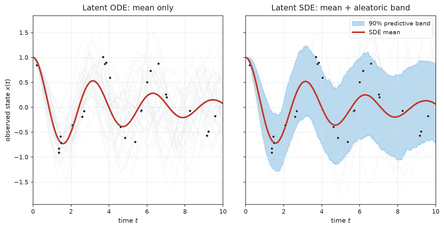
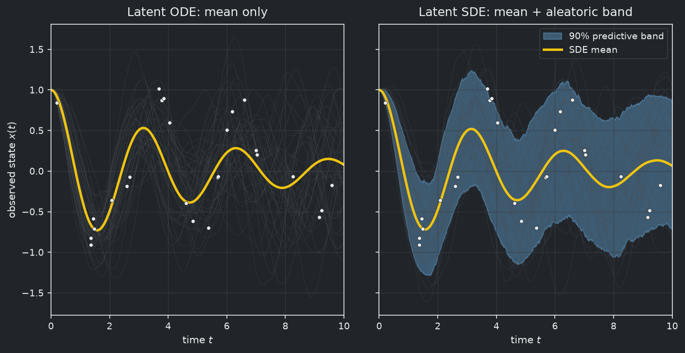
For a lot of physical, biological, and financial processes that third source of uncertainty is the dominant one. A latent SDE can separate the three. The posterior over \(z_0\) gives you initial-condition uncertainty. The posterior over the drift and diffusion parameters gives you epistemic (model) uncertainty. The diffusion term itself gives you aleatoric (intrinsic) uncertainty. They are three different things and they propagate forward in three different ways. If you care about decision-making under uncertainty (I do, it is kind of the whole point), being able to tell them apart is worth a great deal.
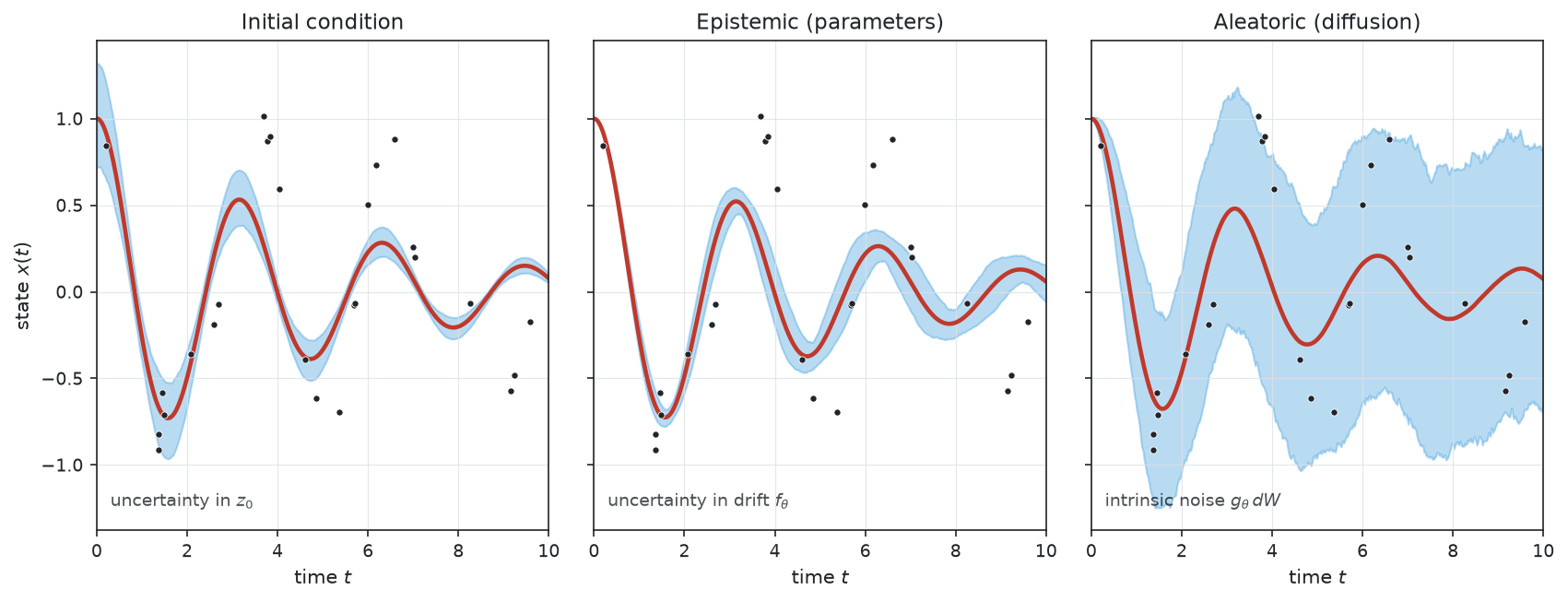
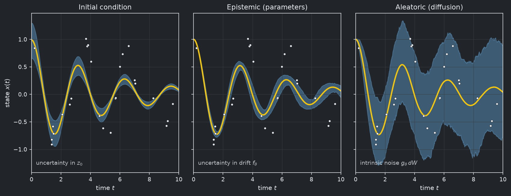
There is also a modeling payoff here. If you fit a deterministic model to a process that is actually stochastic, the model will either overfit the noise or smear it into the drift in weird ways. The diffusion term gives the noise a sanctioned place to live, so the drift can focus on the actual mean dynamics. This is the same reason a Gaussian likelihood beats an L2 loss in a regression with non-degenerate noise: you stop forcing the model to pretend the noise is signal.
Training: the awkward bit
I would be lying if I said training these was as easy as training a ResNet. It is not. There are two and a half headaches.
Headache one: you cannot just backprop through an SDE solver the way you can through an ODE solver, because the Brownian increments are not differentiable functions of the parameters in the usual sense. The clean fix is the adjoint sensitivity method extended to SDEs, which is what (Li et al. 2020) gives you. You integrate the SDE forward, store what you need, integrate an adjoint process backward, and recover gradients with respect to drift and diffusion parameters. Memory-cheap, which matters when your time series is long. The Diffractor-style libraries and the Julia SDE ecosystem handle this; in Python, torchsde is the reference implementation.
There is a newer escape hatch worth knowing about: simulation-free training. SDE Matching (Bartosh et al. 2025) borrows the score- and flow-matching trick from generative modeling and applies it to latent SDEs, skipping the costly numerical simulation entirely. I have not tried it yet, but it is the direction I would look first if I were scaling this up today.
Headache two: the diffusion network \(g_\theta\) is famously hard to train by pure likelihood maximization because the diffusion appears inside an expectation and its gradient is high variance. Two common escapes. One, the GAN approach from (Kidger et al. 2021): train a discriminator over paths and let it push the generated path distribution toward the data path distribution. Two, a fixed or lightly-trained diffusion with the drift carrying most of the learned structure. In practice I lean toward the second for a first pass: fix \(g\) to something reasonable (or learn it slowly with a small learning rate), get the drift right, then let \(g\) adapt. The drift is where most of your useful signal lives anyway.
Headache two and a half: reparameterization tricks for SDEs are subtler than for VAEs because the noise is correlated across time in a structured way. Read (Tzen and Raginsky 2019) carefully before you roll your own. I did not, the first time, and I got a model that trained beautifully and produced uncertainty bands that were completely miscalibrated. Fun times.
A sketch in Julia
I promised myself I would stop writing blog posts with code I have not run. I am going to bend that rule here and show a sketch, with the explicit caveat that the version I actually trust is the one I will commit to the repo after this post goes up. Consider this pseudocode with correct shape.
using Lux, Random, DifferentialEquations, DiffEqSensitivity, Distributions

# Drift and diffusion networks. The diffusion must produce a non-negative
# scale, so we softplus the output.
drift = Chain(Dense(d, 64, tanh), Dense(64, d))
diffusion = Chain(Dense(d, 64, tanh), Dense(64, d), x -> softplus.(x))

# The latent SDE right-hand sides.
function f(u, p, t)
    drift_u, _ = Lux.apply(drift, u, p.drift, nothing)
    return drift_u
end

function g(u, p, t)
    _, diff_u = Lux.apply(diffusion, u, p.diff, nothing)
    return diff_u .* I(d)  # diagonal diffusion for sanity
end

# Encoder: map the observation sequence to (mean, logstd) of z0.
encoder = Chain(Dense(obs_dim * T, 128, tanh), Dense(128, 2d))
mu_logstd(encoder_out) = (encoder_out[1:d], encoder_out[d+1:end])

# Decoder: map latent state at time t to observation likelihood params.
decoder = Chain(Dense(d, 64, tanh), Dense(64, obs_dim))

# Forward: sample z0 ~ q(z0 | x), integrate the SDE, decode at observed times.
function elbo(x, ts, params, rng)
    enc_out = Lux.apply(encoder, x, params.enc, nothing)[1]
    mu, logstd = mu_logstd(enc_out)
    z0 = mu .+ exp.(logstd) .* randn(rng, d)

    prob = SDEProblem(f, g, z0, (ts[1], ts[end]), params)
    sol = solve(prob, EulerHeun(), saveat=ts, dt=0.01)

    # Reconstruction: Gaussian likelihood at each timestep.
    recon = 0.0
    for (i, t) in enumerate(ts)
        dec_out = Lux.apply(decoder, sol.u[i], params.dec, nothing)[1]
        recon += logpdf(MvNormal(dec_out, 0.1), x[:, i])
    end

    # KL between q(z0) and a standard Gaussian prior. The path KL is
    # approximated by the initial-state KL plus a correction term; see
    # Tzen & Raginsky (2019) for the full thing.
    kl = 0.5 * sum(exp.(2 .* logstd) .+ mu .^ 2 .- 1 .- 2 .* logstd)

    return recon - kl
end
The shape is right. The training loop, the adjoint setup, and the path-KL correction are what I still need to nail down before I would call this runnable. Treat it as a map of the territory.
Where I would actually use this
A few places where latent SDEs are worth the complexity, in my opinion:
Irregularly sampled clinical pharmacokinetics, where you have a few plasma concentrations per patient at weird times and you want a model that handles the gap structure without imputation theatre. The continuous-time nature of the SDE is doing real work here, not just looking good on a slide.
Financial return series where you suspect the volatility itself is a stochastic process (so, basically all of them). A latent SDE with a learned diffusion gives you a learned stochastic volatility model that is not wedded to the Heston parametric form. Whether that trades well is a different question, but the modeling surface is richer.
Sensor networks with dropout, where a device goes offline for an hour and comes back. You just do not decode during the offline window and the SDE bridges the gap with a properly widening uncertainty band. That widening band is the model telling you the truth, which is that it is less sure the longer the gap. I find this genuinely moving as an engineering property. The model knows what it does not know.
Forecasting with safety-critical downstream decisions, where a calibrated smear beats a confident point. If you are going to act on the forecast, you need the uncertainty to be part of the artifact.
For clean, regularly sampled, low-noise data where you only need the mean, a latent SDE is overkill. Use a latent ODE or even just a sequence model. The SDE tax is real and you should only pay it when the noise is the point.
Conclusion
Latent SDEs are the model I reach for when I want a neural time-series model that takes uncertainty seriously in all three directions: where it started, what it is, and how it kicks. They are not the easiest model to train, and I would not recommend them as a first resort. But for messy, irregular, intrinsically stochastic processes, they are the most honest object in the toolbox. The diffusion term gives the noise a home, the latent structure keeps the dynamics low-dimensional and interpretable, and the continuous-time formulation makes irregular sampling a non-issue.
I am still working through the Julia implementation, and I will post the runnable version once I have it.