Introduction
A few months ago I wrote a piece trying to explain World Models (Schmidhuber 1990; Ha and Schmidhuber 2018) and the Joint Embedding Predictive Architecture (JEPA) (Assran et al. 2023). I didn’t provide any code or results in that post. I mainly spoke about the theoretical aspects of world models and how I believe they are a good bet for our next leap in AI.
This time, I want to show you how to build the smallest possible thing that still deserved the name “JEPA world model”. Kind of a toy problem, where I could check whether the latent space was doing what it’s supposed to.
It’s a tutorial that you can follow along with. I’m going to walk you through what a JEPA actually is, in code, in Julia, on a bouncing ball. We’ll peek inside the latent space to see if it learned physics.
If you want the conceptual background first, go read my LinkedIn post on LeWM and come back. If you want to skip the prose and look at the code, it starts in the next section, and every snippet below was run end-to-end, on Julia 1.12 with Flux 0.16, to produce the loss curve and the latent plots you’ll see further down.
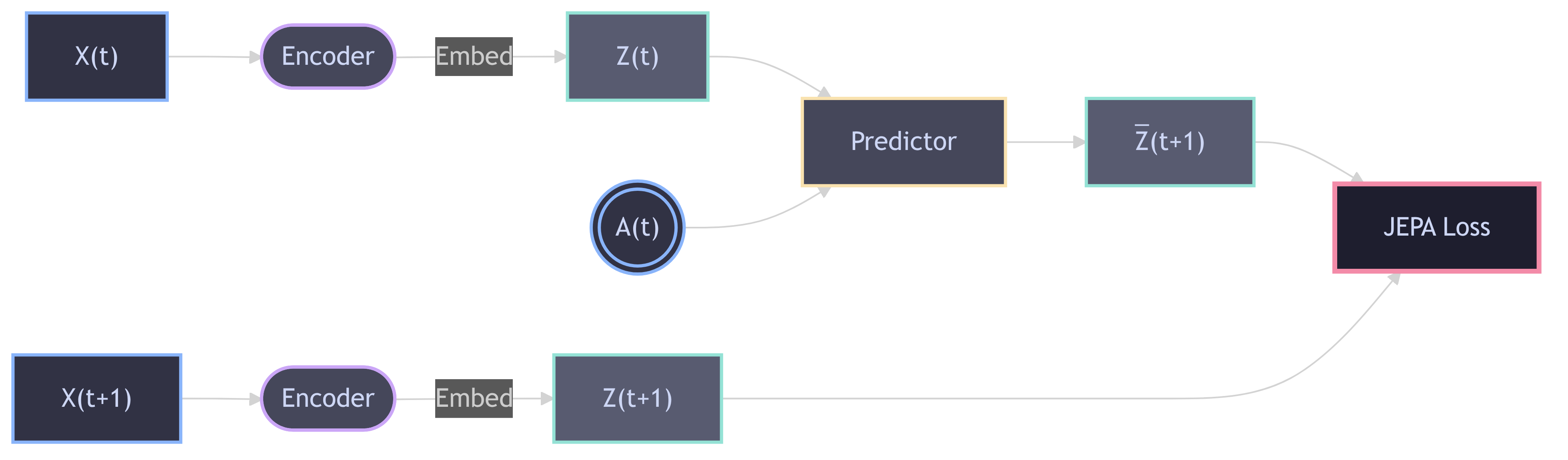
Before jumping in to code I want you to have a conceptual picture in mind outlining what JEPA does. I’ve drawn a diagram in Figure 1. \(X(t)\) is the input at time \(t\), \(Z(t)\) is the latent space at the same time and Encoder is the neural network mapping the input \(X\) to latent \(Z\). Predictor is another neural network taking an action \(A(t)\) and an embedding \(Z(t)\) and outputs a future latent state represented by the embedding \(\bar{Z}(t+1)\). The JEPA loss then compares the “true” latent state \(Z(t+1)\) with the predicted \(\bar{Z}(t+1)\). Note that the encoder here is the same.
What we are actually building
We’re going to build a ball bouncing in a 1D box, but it could be a pendulum, a cartpole, a video frame stream, the trajectory of a customer churn funnel. The point is, there’s an underlying state (position, velocity) and we only get to see observations of it (the noisy y-coordinate, a pixel, a feature vector).
A “world model” is a system that, given some observations, builds an internal representation of the state and can predict what will happen next. That’s it. That’s the whole ambition. JEPA is a bet on how to build one without falling into the generative-modelling trap (where the model is paid to predict every pixel of the next frame, including the irrelevant ones, and ends up spending all its capacity on texture and noise).
The trick of JEPA is the energy. You don’t try to reconstruct the next observation. You try to make the embedding of the next observation predictable from the embedding of the current one. The loss is embedding-wise rather than pixel-wise, and the model is free to throw away information that doesn’t help prediction.
For a quick note on Energy based models. They’re a super simple way to create a compatability score (Energy) between input output pairs which we typically denote \(E(x, y)\). We can express this probabilistically as
\[p(y|x)=\frac{e^{-E(x,y)}}{Z(x)}\]
where \(Z(x)\) is the partition function that normalizes the probability.
The architecture, in two pieces
Two modules. Both are just MLPs because I want the focus to be on the training objective, not on attention or convolutions. In a serious world model you’d use a backbone appropriate to your data. For a bouncing ball, an MLP is plenty.
struct JEPA{M, P}
    encoder::M     # observation -> latent
    predictor::P   # (latent, action) -> predicted latent
end

function encode(model, x)
    model.encoder(x)
end

function predict(model, z, a)
    model.predictor(vcat(z, a))
end

function jepa_loss(model, x_t, a_t, x_tp1)
    z_t          = encode(model, x_t)
    z_tp1_pred   = predict(model, z_t, a_t)
    z_tp1_target = encode(model, x_tp1)
    return mean(sum((z_tp1_pred .- z_tp1_target) .^ 2, dims=1))
end
Notice that we’re not leveraging a lot of tricks here. No stop-gradient, no detach, no second “target network” trailing the first by a moving average. The target is the live encoder run on the next observation, gradients flowing through it and everything. By the usual story that should collapse instantly: the cheapest way to make z_tp1_pred match z_tp1_target is for the encoder to map every input to the same constant and call it a day. The thing that stops that from happening is the regulariser in the next section, and getting away with only that, no stop-gradient and no EMA, is the whole bet of the LeJEPA (Balestriero and LeCun 2025) and LeWM (Maes et al. 2026) line of work.
Two things worth naming here. The world-model I’m building is closest in spirit to LeWorldModel (LeWM), the recent Maes and Balestriero line that trains a JEPA straight from pixels with exactly two loss terms: a next-embedding prediction loss and a regulariser. That regulariser is SIGReg, introduced in the LeJEPA paper, where the argument is that an isotropic Gaussian is the unique collapse-proof target distribution for a representation like this. If you read one paper, read LeJEPA. If you want to see it scaled to a real world model from pixels, read LeWM. What I’ve got is a tiny cousin of both, in Julia, on a bouncing ball.
The other thing is what I deliberately left out. Everyone’s recipe for “stop the encoder from collapsing” is normally some flavour of teacher-student asymmetry: SimSiam stops the gradient into the target, BYOL and DINO keep a separate target network trailing the online one by a moving average. LeJEPA’s claim, the one I actually wanted to test, is that with a strong enough regulariser you need none of that. So I’m not using any of it. No stop-gradient, no EMA, one network doing both sides of the loss. If the latent stays healthy, SIGReg is the only thing holding it up.
The a_t argument is the action. For our bouncing ball, that’s “is the ball at the top of its arc moving up or down” encoded as a small vector. In a real RL setup the action would be a motor command. In a passive video setup you’d use positional encoding of the timestep instead, because there is no action. We’re going to be on the action side, because it makes the architecture more direct.
There is no decoder. That’s the whole point of the JEPA framing. We are not trying to reconstruct the observation. We are not trying to generate. We are only trying to predict the next embedding.
The regularizer that does the heavy lifting
If you train the network above, it will work. It will collapse a little. The latent space will start filling with junk dimensions and the model will use them as a private scratch pad to memorise trajectories.
This is where SIGReg comes to the rescue. SIGReg stands for Sketched Isotropic Gaussian Regularization, and it comes out of the LeJEPA line of work (Assran et al. 2025; Balestriero and LeCun 2025). The idea is beautifully simple. A good latent space for a world model is one where the distribution of embeddings, taken over a batch, is close to an isotropic Gaussian. Same variance in every direction, no covariance between directions. Why? Because an isotropic Gaussian is the maximum-entropy distribution under a fixed second moment, so it’s the one that throws away the least information while staying collapse-resistant. A JEPA trained with a SIGReg penalty is being asked to learn a representation whose batch statistics are as “spread out” as possible without privileging any axis.
The “sketched” part is how you check that cheaply. Measuring the full distribution of a 16-dimensional latent every step is hopeless, so SIGReg picks a few hundred random directions, projects the batch onto each, and asks a one-dimensional question instead: does this projection look like a standard normal? If every random 1D shadow of the cloud is N(0, 1), the cloud itself is an isotropic Gaussian. The clever part is how it tests a projection. Instead of just checking the variance, it compares the projection’s empirical characteristic function (the average of cos(t·x) and sin(t·x) over the batch, at a handful of frequencies t) against the characteristic function of a standard normal, exp(-t²/2). That’s the Epps-Pulley Gaussianity test, and it catches the mean, the variance, and the shape all at once. The penalty looks like this:
const KNOTS = collect(range(0f0, 3f0, length=17))   # frequencies to test the CF at
const PHI   = exp.(-KNOTS .^ 2 ./ 2)                # standard-normal characteristic fn
const SW    = simpson_weights(KNOTS)                # quadrature weights on [0, 3]

function sigreg(z; n_proj=256)
    D, B = size(z)                                  # z: (latent, batch)
    A = randn(Float32, D, n_proj)
    A = A ./ sqrt.(sum(A .^ 2, dims=1))
    # compute the epps-pulley statistic (Here be dragons...)
    x  = A' * z                                     # (n_proj, batch)
    xt = reshape(x, n_proj, B, 1) .* reshape(KNOTS, 1, 1, :)
    re = dropdims(mean(cos.(xt), dims=2), dims=2)
    im = dropdims(mean(sin.(xt), dims=2), dims=2)
    err = (re .- reshape(PHI, 1, :)) .^ 2 .+ im .^ 2
    mean(err * SW)
end
Why this is enough to replace the stop-gradient: think about what the trivial collapse actually looks like. If the encoder maps every input to the same point, every projection becomes a spike at one value, and the characteristic function of a spike is a flat line at one, nothing like the exp(-t²/2) bell. SIGReg sees that immediately and slams it. The imaginary (sin) part pins the mean to zero, the real part pins the variance and the shape. There’s no comfortable degenerate solution left for the prediction loss to run to, so the encoder has to actually spread out and stay spread out. That’s the LeJEPA result in one sentence: a strong enough distributional regulariser does the job the stop-gradient was hacking around.
It comes with exactly one knob, the weight on the SIGReg term:
loss = pred_loss + λ * sigreg(z_t) # λ = 1 throughout. that's the whole schedule.I set λ = 1 and never touched it. No warmup, no decay, no per-layer tuning. That’s the part the LeWM abstract is quietly proud of: it takes a method that used to carry six loss-balancing hyperparameters down to one.
Bouncing ball, in 200 lines
We are generating the trajectories of a ball under constant gravity, bouncing off a floor at x=0 and keeping a fraction e of its speed each bounce.
function simulate_ball(; n_steps=200, dt=0.05, g=9.81, x0=0.0, v0=5.0, e=0.9)
    x = zeros(n_steps); v = zeros(n_steps)
    x[1], v[1] = x0, v0
    for t in 1:n_steps-1
        xn = x[t] + v[t]*dt - 0.5*g*dt^2
        vn = v[t] - g*dt
        if xn < 0
            # solve x[t] + v[t]·τ − ½g·τ² = 0 for the crossing time τ ∈ (0, dt]
            a = -0.5*g; b = v[t]; c = x[t]
            sq = sqrt(max(b^2 - 4a*c, 0.0))
            τ  = minimum(t_ for t_ in ((-b+sq)/(2a), (-b-sq)/(2a)) if t_ > 1e-12)
            v_impact = v[t] - g*τ                   # velocity at contact (downward)
            v_after  = -e * v_impact                # we need to lose a bit of speed
            rem = dt - τ                            # finish the step from the floor
            xn = v_after*rem - 0.5*g*rem^2
            vn = v_after - g*rem
            if xn < 0; xn = 0.0; vn = e*abs(vn); end
        end
        x[t+1] = xn; v[t+1] = vn
    end
    return x, v
end
I actually had a funny bug in this simulation in the beginning where the ball magically received extra energy after bouncing. But yeah, the code above should be good to go.
using CairoMakie

dt = 0.01
x, v = simulate_ball(; n_steps=550, dt=dt, v0=5.0)
ts = (0:length(x)-1) .* dt
xmax = 1.1 * maximum(x)

fig = Figure(size = (820, 380))
axb = Axis(fig[1, 1], title = "Bouncing ball", ylabel = "height x", limits = ((-1, 1), (-0.05, xmax)))
hidexdecorations!(axb)
lines!(axb, [-1, 1], [0, 0], color = :black, linewidth = 2)         # the floor
ball = Observable(Point2f(0, x[1]))
scatter!(axb, ball, markersize = 28, color = :crimson)

axt = Axis(fig[1, 2], title = "Height vs time", xlabel = "time (s)", ylabel = "height x",
           limits = ((0, ts[end]), (-0.05, xmax)))
trace = Observable(Point2f[(ts[1], x[1])])
lines!(axt, trace, color = :crimson, linewidth = 2)

record(fig, "figs/bounce.gif", 1:length(x); framerate = 60) do i
    ball[]  = Point2f(0, x[i])
    trace[] = Point2f.(ts[1:i], x[1:i])
end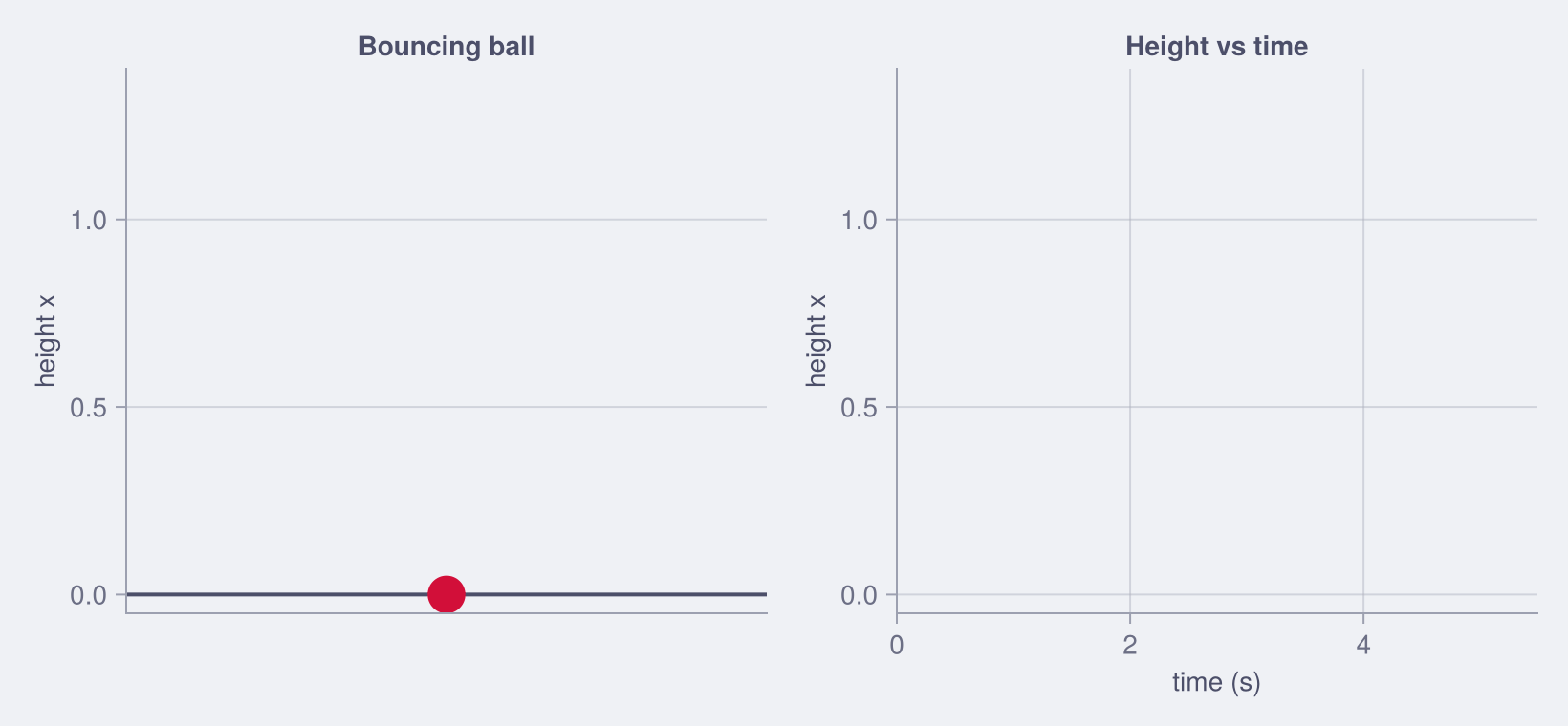
Each arc is a parabola, each bounce peak is 0.9× the energy of the one before, and nothing ever goes below the floor. That’s the world the JEPA has to figure out, except it never sees x and v; it sees only the noisy height. Don’t mind the speed here.. I know it’s like it’s bouncing on the moon but it really doesn’t matter for our case here.
The observation is x corrupted with Gaussian noise. The latent we’d like to recover is the true state (x, v). The model never sees (x, v) directly, and here is a subtlety that turns out to matter enormously, so I’ll flag it now and pay it off later: a single height tells you nothing about velocity. The ball passes through any given height twice, once going up, once coming down, at opposite-sign velocities, and different throws pass the same height at different speeds. So if the encoder’s input is one frame, velocity is simply not a function of that input. It is unrecoverable in principle, not just in practice.
The standard approach here is to give the encoder a short stack of recent frames instead of one. From a window of consecutive heights you can infer velocity (it’s roughly the finite difference). So the observation I feed the encoder is the last K=4 noisy heights; the action is the sign of the velocity, sign(v[t]), handed to the predictor; and the true (x, v) is kept aside, never fed in, purely to probe the latent afterwards.
function sample_batch(batch; n_steps=200)
    obs   = zeros(Float32, batch, n_steps)   # noisy heights (what the encoder sees, windowed below)
    xtrue = zeros(Float32, batch, n_steps)   # clean position (probe only)
    vtrue = zeros(Float32, batch, n_steps)   # true velocity  (probe only)
    acts  = zeros(Float32, batch, n_steps)   # action = sign(v)
    for b in 1:batch
        v0   = 3.0 + 4.0 * rand()            # random launch speed
        x, v = simulate_ball(; n_steps=n_steps, v0=v0)
        obs[b, :]   .= Float32.(x) .+ 0.05f0 .* randn(Float32, n_steps)
        xtrue[b, :] .= Float32.(x)
        vtrue[b, :] .= Float32.(v)
        acts[b, :]  .= Float32.(sign.(v))
    end
    return obs, xtrue, vtrue, acts
end
The training loop (next section) slides a length-K window over each trajectory to build the inputs. The observation at time t is obs[b, t-K+1:t], and the prediction target is the window one step later. The latent is 16-dimensional, not because the state needs 16 numbers (it needs two), but because I learned the hard way not to bottleneck it; more on that when we probe. If the world model is doing its job, those 16 dimensions should between them lay out the full (position, velocity) state, even though the model is never told those two things exist.
The training loop
using Flux, Statistics, Random, LinearAlgebra

function train_jepa(; n_epochs=40, n_traj=400, batch=256, latent=16, lr=1e-3, K=4, λ=1f0)
    encoder   = Chain(Dense(K, 32, relu), Dense(32, latent))   # input = K-frame window
    predictor = Chain(Dense(latent + 1, 32, relu), Dense(32, latent))

    # Pool every (window_t, action, window_{t+1}) transition once, then shuffle.
    # The K-frame window is what makes velocity observable; the pool-and-shuffle is
    # just ordinary SGD, and it matters because looping over timesteps in trajectory
    # order marches every ball through the arc in lockstep, and those correlated
    # gradients make training thrash.
    obs, xtrue, vtrue, actions = sample_batch(n_traj)
    B, T = size(obs)
    nwin = B * (T - K)
    W_t = zeros(Float32, K, nwin); W_tp1 = zeros(Float32, K, nwin); A_t = zeros(Float32, 1, nwin)
    i = 0
    for b in 1:B, t in K:(T-1)
        i += 1
        @views W_t[:,  i] .= obs[b, t-K+1:t]      # window ending at t
        @views W_tp1[:, i] .= obs[b, t-K+2:t+1]    # window ending at t+1
        A_t[1, i] = actions[b, t]
    end
    N = nwin

    model     = (; encoder, predictor)          # everything we optimise
    opt_state = Flux.setup(Adam(lr), model)

    losses = Float32[]
    for epoch in 1:n_epochs
        order = randperm(N)                     # fresh shuffle each epoch
        epoch_loss = 0.0f0; nbatches = 0
        for s in 1:batch:N-batch
            cols  = order[s:s+batch-1]
            w_t   = W_t[:,  cols]
            a_t   = A_t[:,  cols]
            w_tp1 = W_tp1[:, cols]
            loss, grads = Flux.withgradient(model) do m
                z_t    = m.encoder(w_t)
                z_pred = m.predictor(vcat(z_t, a_t))
                z_tgt  = m.encoder(w_tp1)        # same encoder, gradients flow. no stop-grad, no EMA.
                pred   = mean(sum((z_pred .- z_tgt) .^ 2, dims=1))
                pred + λ * sigreg(z_t)           # SIGReg keeps z_t from collapsing
            end
            Flux.update!(opt_state, model, grads[1])
            epoch_loss += loss; nbatches += 1
        end

        push!(losses, epoch_loss / nbatches)
        epoch % 10 == 0 && @info "epoch=$epoch loss=$(losses[end])"
    end

    return model.encoder, model.predictor, losses
end

# the figures below come from exactly this seed
using Random; Random.seed!(1)
encoder, predictor, losses = train_jepa()
One important point is where SIGReg should live. I started by regularising the predictions and letting the loss sort out the encoder. Bad idea. The encoder happily flattened one of its latent dimensions to near-zero variance and used it as a dead axis, and the prediction loss never complained, because the predictor just learned to route around it. Move SIGReg onto the encoder output z_t, the thing you actually probe later, and the collapse goes away.
Another thing about this is how to batch the trajectories. Doing one timestep at a time, every ball at t=1, then every ball at t=2, and so on seems natural, but actually won’t work well. Every gradient step sees a batch of balls at the same phase of their arc, the updates are wildly correlated, and the loss thrashes. One way to deal with this is the pool-and-shuffle in the loop above. Here is the loss across eight random seeds:
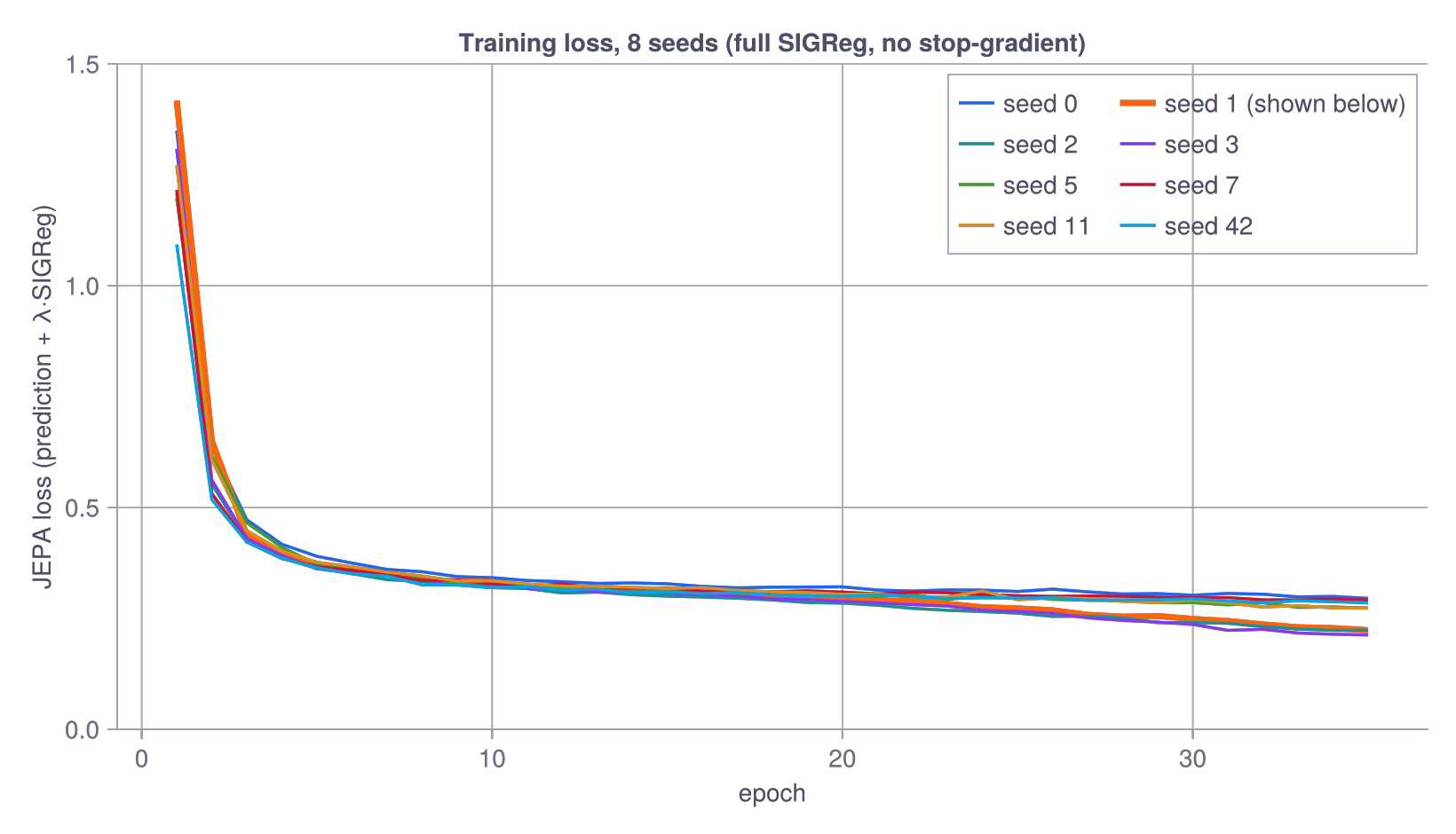
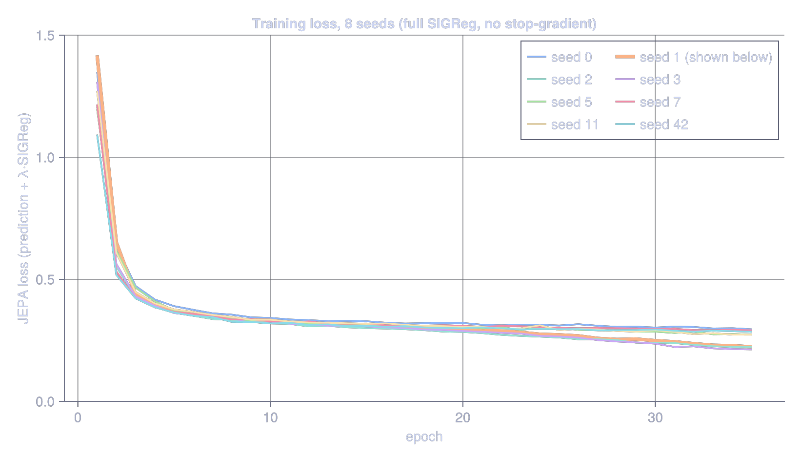
Eight seeds, no stop-gradient, no EMA, one fixed regulariser weight, and the curves are almost indistinguishable. They drop hard for a few epochs, then settle onto the same floor and stay. What makes them land on the same representation, not just the same loss, is giving the latent enough room. I started with a 2-dimensional latent (so I could scatter-plot it without PCA), and there the runs were all over the place, some encoding velocity and some not depending on the seed. Bump it to 16 dimensions, overkill for a state that needs two, and the seed-dependence vanishes: every run recovers position and velocity to within a few percent of the others. I pin seed 1 for the probe figures below, but the pin barely matters here. They all tell the same story.
Peeking inside the latents
First, a yardstick, because otherwise none of the R² numbers below mean anything. The task is easy: from a window of recent heights, position is just the last frame and velocity is roughly the finite difference, both linear functions of the input. A plain supervised linear probe on the raw 4-frame window confirms it, scoring R² 0.99 for position and 0.59 for velocity (velocity caps below 1 only because the 0.05 noise on each frame swamps a one-step difference). So the bar for the self-supervised latent isn’t “can it represent the state in principle” (of course it can). It’s “does a representation trained only to predict its own next embedding recover the state as well as a supervised readout of the raw input?” Hold that 0.99 / 0.59 in mind.
My first version fed the encoder a single frame, one noisy height. I trained it, ran the probe, and got a result that looked deep. Projected onto its top two principal components and coloured by true position, the latent traced a smooth monotonic curve: position cleanly laid out, a linear probe recovering it at R² ≈ 0.99. The same points coloured by velocity were a scrambled mess: a velocity probe scored R² ≈ 0.00, nothing.
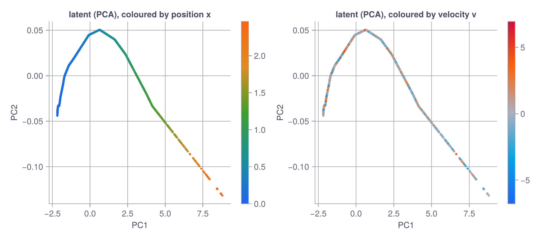
The ball passes every height twice, going up and going down, at opposite-sign velocities, and different throws cross the same height at different speeds. So velocity is not a function of one frame. No encoder, however clever or however many latent dimensions you give it, can extract it from an input that doesn’t contain it. The latent collapses to a curve (you can see it’s effectively rank-one, despite living in 16 dimensions) because the input is effectively one-dimensional.
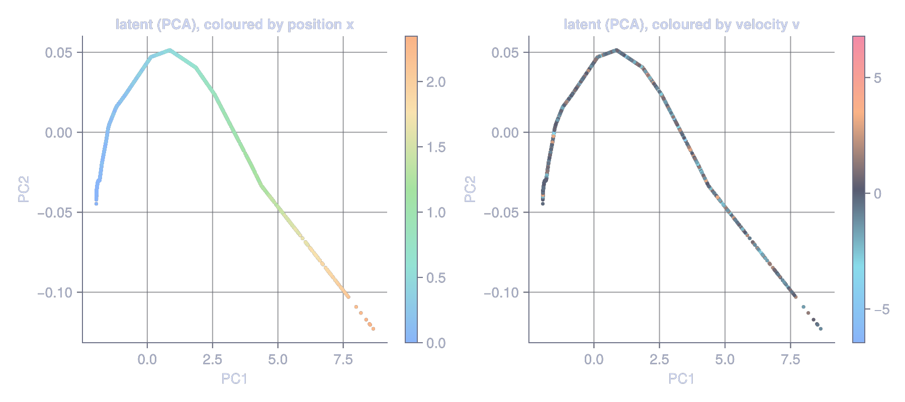
The simple fix is to use the frame window from the data section. Feed the encoder the last four heights, from which velocity is recoverable. Same architecture, same loss, same everything; the only change is Dense(1, …) becomes Dense(4, …). Now the probe tells a completely different story.
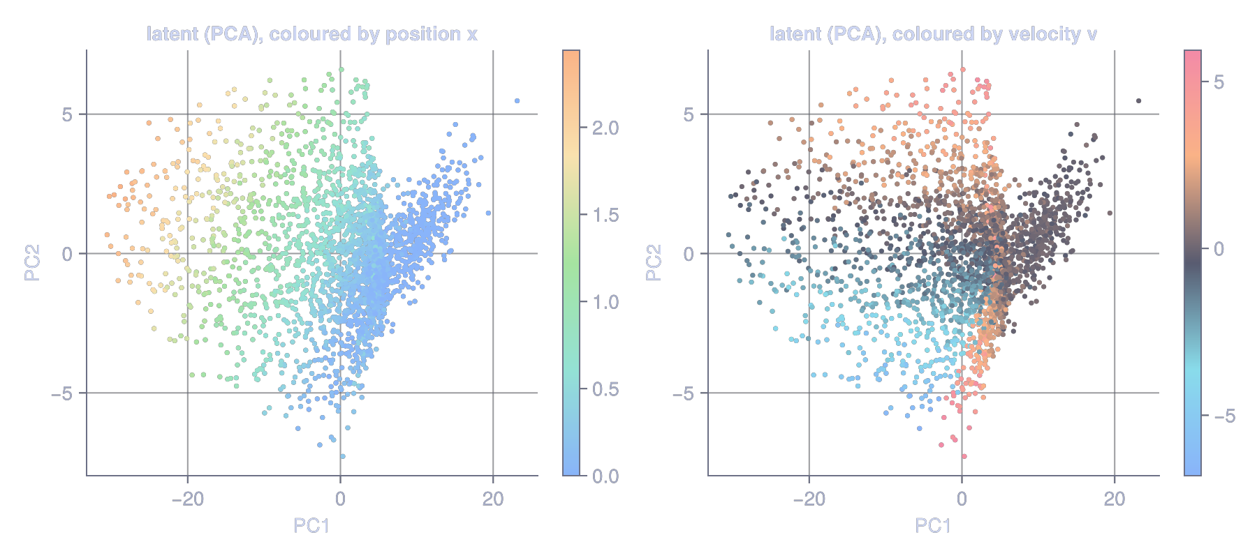
The latent is no longer a curve: it’s a genuinely two-dimensional cloud, and the two colour fields run in roughly perpendicular directions across it: position varies one way, velocity the other. Now hold it up against the yardstick. Position reads out at R² ≈ 0.99, matching the supervised linear probe. Velocity, which was flat-zero in our first attempt, comes back at R² ≈ 0.6, right around the noisy linear ceiling of 0.59. A representation trained with no labels at all, no stop-gradient, no EMA, only next-embedding prediction against a distributional regulariser, reconstructs the full (position, velocity) state about as well as a supervised readout of the raw input. And it’s steady across seeds. Every one lands at position ≈ 0.99 and velocity in the high 0.5s to high 0.6s.
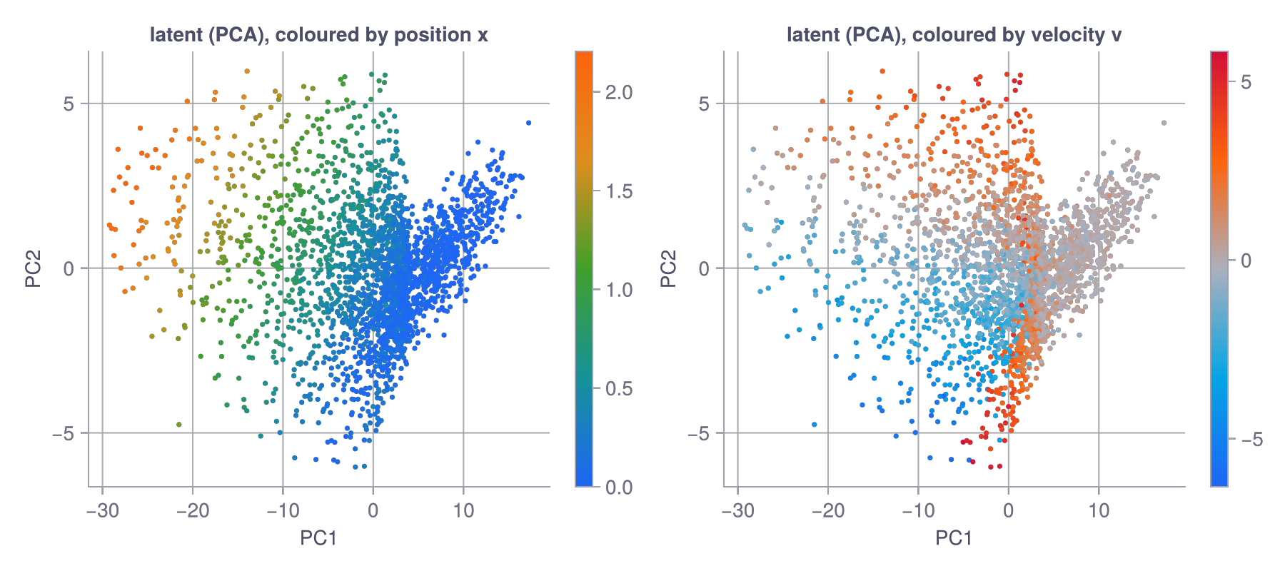
Those panels are a flat projection, though, and the cloud has more than two dimensions worth of structure. Here’s the same latent in its top three principal components, live.
This is cool since you can clearly see two planes in the 3D plot which makes sense since we need two for position and velocity.
Why care about a toy problem?
Now, of course the bouncing ball is a toy, the encoder is an MLP, the whole thing trains in 60 epochs on a CPU, and none of it is going to drive a robot, but it at least verifies that the theory checks out.
“World model” sounds like a magic phrase, and when you build one and it’s an encoder, a predictor, and a regulariser. No stop-gradient, no target network, no momentum schedule. You can write it in an afternoon.
A world model is only ever as good as its observations. No loss function or clever regulariser is ever going to recover what isn’t in there. In our case a wider window did. “Make sure your observation actually determines the state you want” is unglamorous, it’s the sort of plumbing the frame-stack in every Atari agent quietly handles, and it was the whole ballgame here.
What I would do next
The obvious one is pushing velocity up. It lands around 0.6, right at the noisy linear ceiling, but I’m still handing the predictor sign(v) as an action, which lets the latent off the hook for the rest. Drop the action, or make the dynamics actually demand velocity magnitude (a little air resistance would do it), and the latent should be forced to carry a cleaner velocity axis. I’d like to watch that R² climb toward the position one as the incentive does.
Then a pendulum instead of a ball. Its state is still (angle, angular velocity), but the geometry wraps around, so the natural latent is a cylinder rather than a sheet. With the frame-window lesson banked, the question is whether the JEPA lays that cylinder out as cleanly as it laid out (x, v) here.
There’s also the isotropy itself. SIGReg is supposed to drive the embeddings to a standard Gaussian, but if I actually look at the per-axis variances of the trained latent they’re all over the place, some squashed, some inflated. The representation works anyway, which suggests λ = 1 is buying me “not collapsed” without buying me “actually N(0, I)”. Turning the weight up, or training longer, should tighten that, and I’d like to know whether a genuinely isotropic latent reads out any cleaner.
And the real version: pixels, a ViT encoder, and an actual control environment, which is what LeWM does. The whole point of the paper is that this heuristic-free recipe holds at that scale. I’ve only shown it survives contact with a bouncing ball. The interesting test is whether the same “no stop-gradient, one regulariser” story still stands when the encoder is 15M parameters and the input is an image.
Conclusion
The world is, mostly, a thing that has more state than it shows you. A world model is a system that builds a representation of the state from observations and uses it to predict. A JEPA is one way to do that, in the embedding space instead of the observation space. The architecture is small, and the whole trick is the regulariser: get the distribution of the embeddings right and the collapse problem that the stop-gradient was invented to dodge simply doesn’t show up.
If you want to try this, the Flux code is straightforward to adapt to Lux, or even PyTorch. The hyperparameters matter but they are forgiving.
If you spot a mistake, in the code, in the math, in the intuition, please reach out.